Tutorial: Stellarator FCI Turbulence — Closed vs Open Field Lines
This tutorial goes from a genuinely non-axisymmetric analytic geometry to
4-field interchange turbulence movies, closed and limiter-open. It follows
examples/stellarator/rotating_ellipse_fci.py
(geometry and FCI operator verification) and
examples/stellarator/stellarator_turbulence.py
(the turbulence runs), explaining every parameter. Background:
Rotating-Ellipse FCI,
Solvers and Design Decisions (why FCI, the phi
solver), and Models and Governing Equations (the
4-field equations).
1. The rotating-ellipse geometry
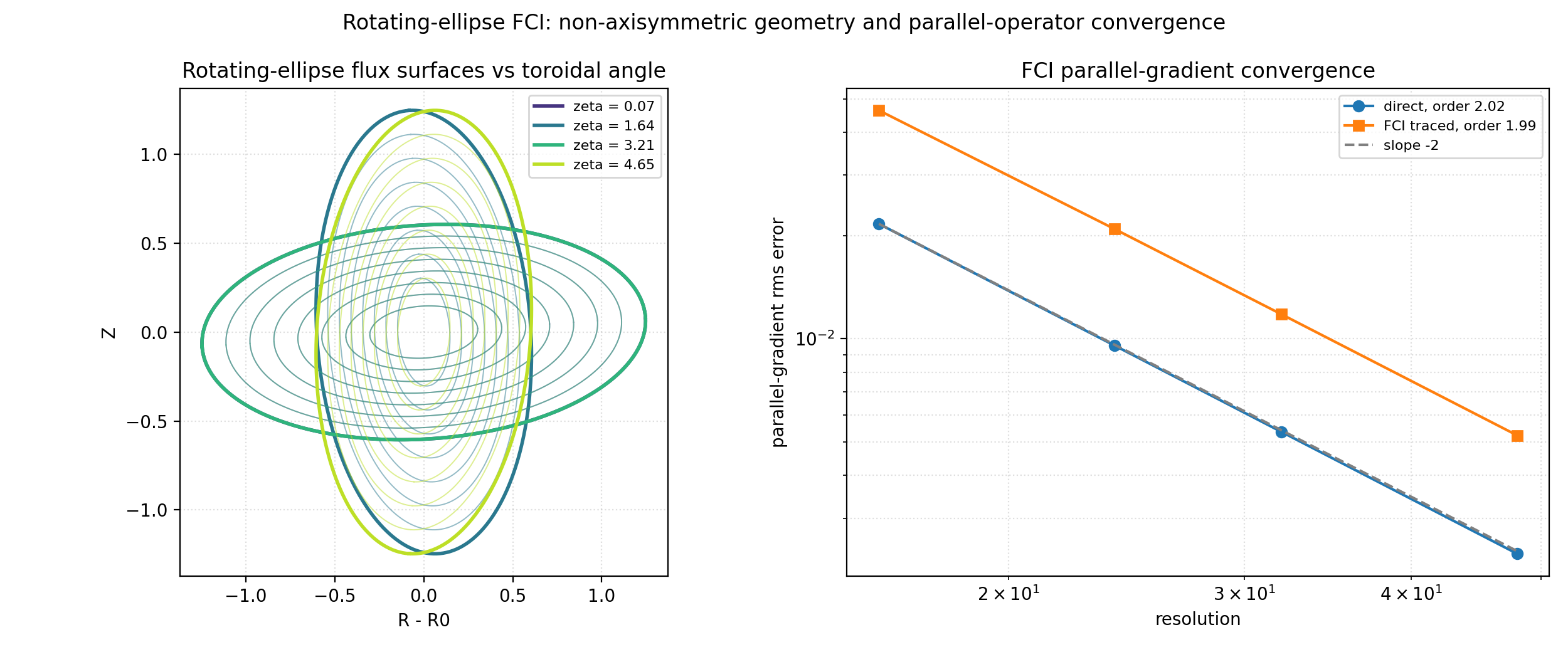
The classical rotating-ellipse (l = 2) stellarator is a torus whose
elliptical cross-section rotates as you follow it toroidally — the canonical
minimal non-axisymmetric field: its metric depends on all three logical
coordinates. In drbx you never derive that metric by hand:
from drbx.geometry import build_rotating_ellipse_geometry

geometry = build_rotating_ellipse_geometry(
    SHAPE,                  # (radial, poloidal, toroidal) cells
    r0=3.0,                 # torus major-radius offset
    elongation=0.35,        # ellipse deformation; aspect ratio (1+d)/(1-d)
    n_field_periods=1,      # ellipse rotations per toroidal turn
    iota=0.9,               # rotational transform of the helical field lines
)
The builder supplies only the analytic embedding
\((x, \theta, \zeta) \mapsto (X, Y, Z)\);
metric_from_position_fn (geometry/embedding.py)
computes \(g_{ij} = \partial_i \mathbf X \cdot \partial_j \mathbf X\), the
Jacobian, and the inverse metric exactly with jax.jacfwd. Because the
metric is built by autodiff, the geometry is itself differentiable with
respect to elongation, iota, etc. (gate:
tests/test_rotating_ellipse_fci.py).
Parameter notes: iota = 0.9 gives strongly helical field lines without a
low-order rational surface inside the tube; elongation = 0.35 is a visibly
non-circular but well-conditioned cross-section; n_field_periods = 1 makes
one full ellipse rotation per toroidal turn.
2. Verifying the FCI operators before doing physics
FCI parallel operators follow field lines between neighboring toroidal
planes and interpolate — no field-aligned coordinates, hence no coordinate
singularities. Before running turbulence, verify the operator order on the
target geometry.
rotating_ellipse_fci.py
does a manufactured-solution refinement over RESOLUTIONS = (16, 24, 32, 48)
with the test field \(\cos(m\theta - n\zeta)\) (MMS_M, MMS_N = 2, 1 — a
low-order helical mode the coarsest grid still resolves), comparing
- the direct operator \(b^i \partial_i f\) (
grad_parallel_op_direct), and - the traced-field-line operator (
grad_parallel_op_fci,MAP_SUBSTEPS = 8tracer substeps between planes)
against the analytic parallel gradient. Both converge at second order — the right panel of the figure above. Run:
PYTHONPATH=src python examples/stellarator/rotating_ellipse_fci.py
3. The 4-field turbulence runs: closed, then limiter-open
stellarator_turbulence.py
runs the interchange model (density, vorticity, ion/electron parallel
velocity — equations on
Models and Governing Equations) twice on the same
rotating ellipse:
closed_geometry = build_rotating_ellipse_geometry(SHAPE, r0=R0,
    elongation=ELONGATION, n_field_periods=NFP, iota=IOTA)
open_geometry = build_rotating_ellipse_geometry(SHAPE, r0=R0,
    elongation=ELONGATION, n_field_periods=NFP, iota=IOTA,
    limiter_radius=0.6)          # flux surfaces with x > 0.6 hit the limiter
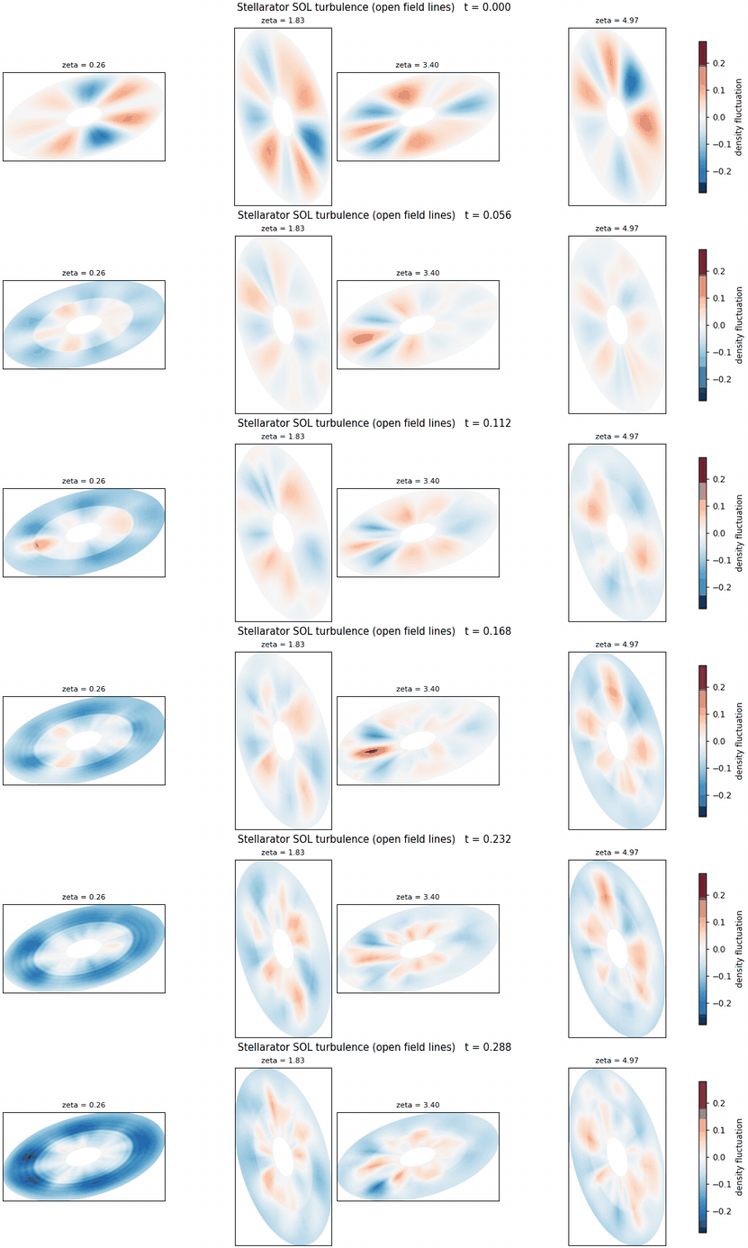
limiter_radius is the only difference: beyond x = 0.6 a toroidal limiter
opens the outer flux surfaces into a scrape-off layer, and the FCI maps grow
target endpoints there. SHAPE = (20, 32, 12) is a laptop-sized grid — the
poloidal direction gets the most cells because the seeded modes are poloidal.
The operator scaffold, built once
parameters = Fci4FieldBlobParameters(
    rho_star=1.0,               # drift scale: interchange drive strength
    phi_inversion_tol=5.0e-5,   # GMRES tolerance of the phi solve
    phi_inversion_maxiter=100,  # per-stage iteration cap
    phi_inversion_restart=200,  # GMRES restart length
)
stencil_builder = LocalStencilBuilder(build_local_stencil_from_field.build_fn)
conservative_builder = ConservativeStencilBuilder(build_conservative_stencil_from_field.build_fn)
boundary_conditions = build_free_decay_boundary_conditions(geometry)
curvature = build_curvature_coefficients(geometry, periodic_axes=(False, True, True))
projectors = build_perp_laplacian_face_projectors(geometry)
phi_solver = build_four_field_phi_solver(
    geometry, parameters,
    conservative_stencil_builder=conservative_builder, face_projectors=projectors)
Everything expensive — stencil builders, curvature coefficients, face
projectors, the GMRES phi solver with its cached jitted closure — is built
once per geometry and reused every stage ("build once, solve many", see
Solvers and Design Decisions). The phi tolerance
5e-5 is loose enough to be fast and tight enough that the movie-scale
dynamics do not change if you tighten it; restart=200 effectively makes the
solve full-memory GMRES at this grid size.
The seeded initial state
envelope = np.sin(np.pi * (x - x.min()) / (x.max() - x.min()))
for m, n in MODES:                 # ((2,1), (3,2), (4,1), (5,3))
    perturbation += rng.uniform(0.5, 1.0) * np.cos(m*theta + n*zeta + random_phase)
state = Fci4FieldState(
    density=1.0 + AMPLITUDE * envelope * perturbation,   # AMPLITUDE = 0.08
    omega=zeros, v_ion_parallel=zeros, v_electron_parallel=zeros)
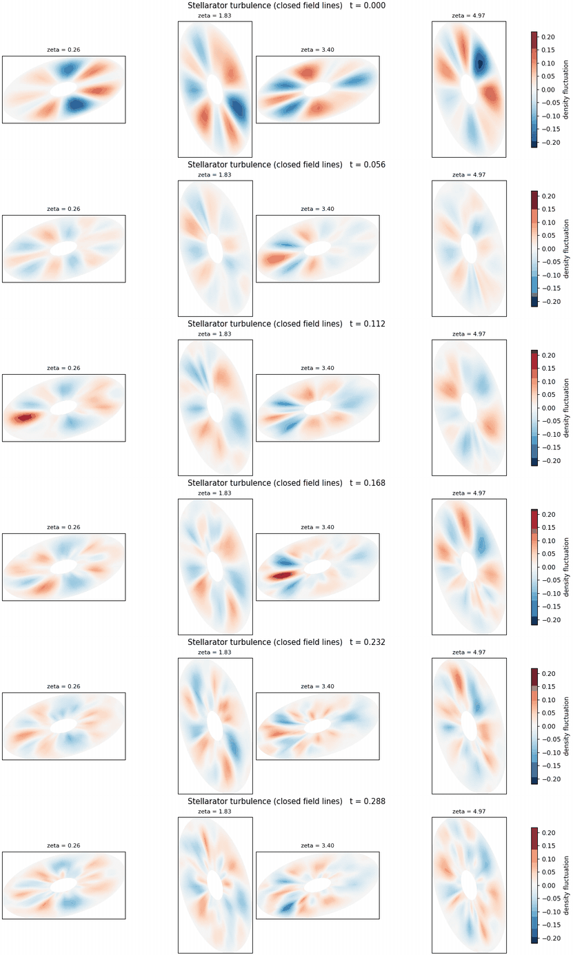
Only the density is perturbed (8% peak, several helical modes with random phases, a radial sine envelope vanishing at the walls): the curvature drive must generate the vorticity itself — that is the interchange mechanism, and it makes the early frames physically meaningful rather than an artifact of a hand-crafted flow.
The stepping loop
for step_index in range(1, STEPS + 1):        # STEPS = 144, DT = 2e-3
    state, phi_guess = four_field_rk4_step(
        state, geometry=geometry, timestep=DT, parameters=parameters,
        curvature_coefficients=curvature, stencil_builder=stencil_builder,
        conservative_stencil_builder=conservative_builder,
        boundary_conditions=boundary_conditions, phi_face_projectors=projectors,
        phi_inverse_solver=phi_solver, phi_guess=phi_guess)

    if use_sheath:   # open geometry only
        sheath = compute_fci_sheath_recycling(state.density, Te, Ti, geometry.maps)
        state = state with density - DT * sheath.ion_particle_loss (floored)
Two things to notice:
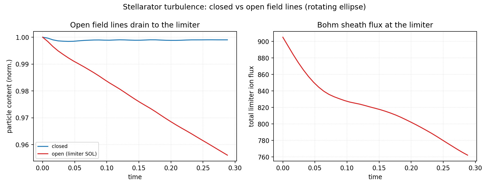
phi_guessis carried between steps: each RK4 stage's perpendicular Laplacian inversion warm-starts from the previous solution, cutting the GMRES iteration count substantially.- On the open geometry the Bohm sheath sink
n c_sis applied explicitly on the limiter endpoint cells after each step — open field lines drain. The run records total particle content and total limiter flux, and the summary figure shows exactly the expected contrast: closed content is conserved, open content decays into the sheath.
DT = 2e-3 satisfies the interchange CFL at this drive; 144 steps with a
frame every 4 steps gives a ~36-frame GIF of the density fluctuation in four
rotating physical cross-sections. Completed runs are cached in
closed_frames.npz / open_frames.npz, so re-rendering movies does not
re-run the physics.
PYTHONPATH=src python examples/stellarator/stellarator_turbulence.py
4. Variations
- Island divertor: replace the geometry with
examples/stellarator/island_divertor.py— a resonant perturbation creates a chain of islands and an emergent stochastic SOL. - 3-D rendering:
examples/stellarator/stellarator_3d_render.pydraws the turbulence on the traced flux surfaces (media/stellarator_3d_turbulence.gif). - Differentiable flux tube:
examples/stellarator/fci_differentiable.pyand Differentiable FCI Flux Tube take gradients through the FCI geometry itself. - Imported equilibria: swap the analytic ellipse for ESSOS coil fields or
VMEX equilibria (
examples/geometry-3D/essos-field-lines/,examples/geometry-3D/vmex/); see ESSOS Field-Line Import.
Gates for this tutorial: tests/test_rotating_ellipse_fci.py,
tests/test_stellarator_turbulence.py, tests/test_island_divertor.py,
tests/test_multigrid_preconditioner.py.