Performance And Differentiability¶

This page records the current fast paths, the current differentiable paths, and the reproducible profiling workflow.

Measured Turbulence Performance¶

The core closed-field-line drift-wave turbulence model (Hasegawa-Wakatani, FFT-spectral RK4) is jit-compiled and differentiable end-to-end. Two measured numbers quantify the "fast and differentiable" claim:

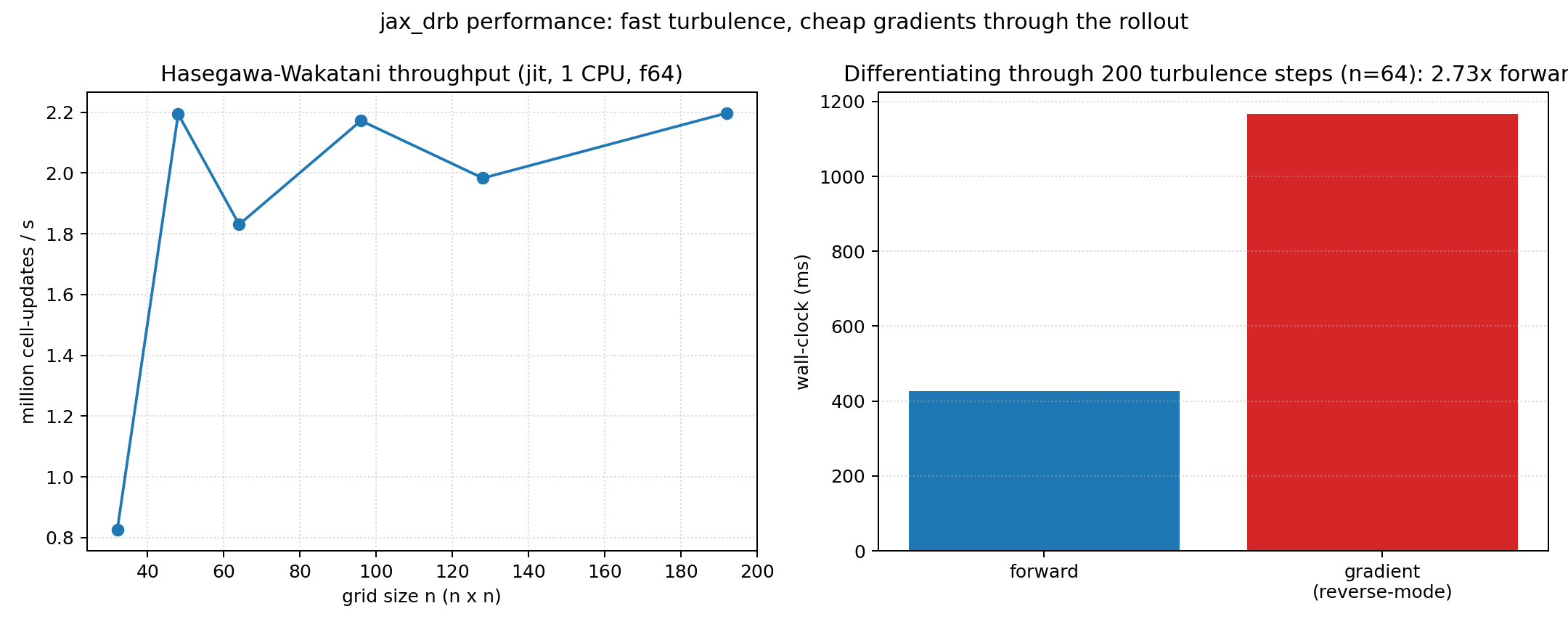
• Throughput is roughly grid-size-independent at about 2 million cell-updates per second on a single CPU in float64 (each step is a dealiased spectral Poisson bracket); it rises substantially on GPU and in float32.
• Differentiating through the turbulence is cheap. One reverse-mode gradient of a diagnostic of the evolved state with respect to the transport-drive parameter — taken through the entire multi-step rollout — costs only about 2.7x a single forward evaluation (here, 200 steps at n = 64), the expected small constant factor of reverse-mode autodiff rather than a cost that grows with the number of steps.

Regenerate with

PYTHONPATH=src python examples/benchmarks/performance_benchmark.py

Absolute timings depend on the host; the scalings do not.

Choosing a Differentiation Method¶

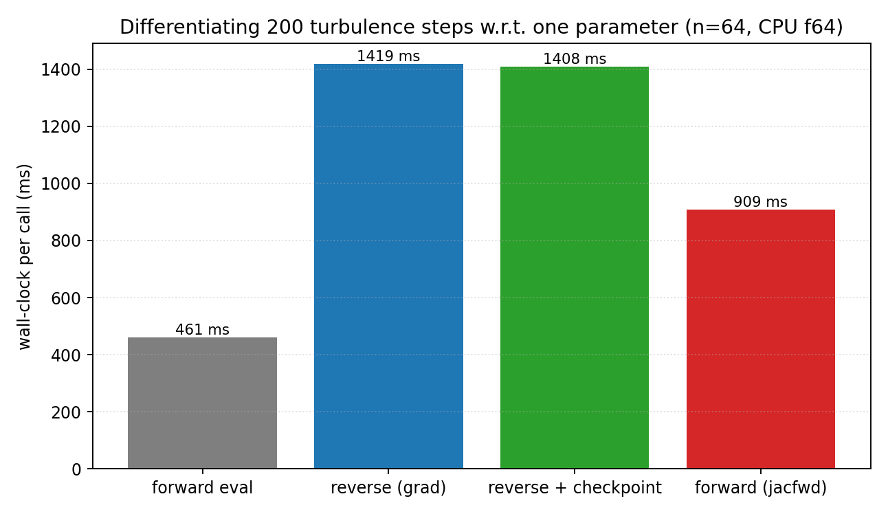
The same gradient can be computed several ways, and the choice changes cost, never the answer (gated to machine agreement in tests/test_autodiff_methods.py). Measured on 200 turbulence steps at n = 64 (one scalar parameter, CPU f64):

• Forward mode (jax.jacfwd) is the most efficient for a few parameters: one tangent rides along the rollout — no reverse sweep, no stored trajectory — costing about 2x a forward evaluation (vs ~3.1x for reverse mode here).
• Reverse mode (jax.grad) wins when differentiating with respect to many parameters at once (fields, geometry): one backward sweep covers them all, at the cost of storing the trajectory.
• Checkpointed reverse (jax.grad + jax.checkpoint on the step) trades a modest recompute for bounded memory — the fix when a long reverse rollout is memory-bound.

Rule of thumb: jacfwd for O(1-10) scalars, grad for parameter fields, add jax.checkpoint when reverse mode runs out of memory. Reproduce with

PYTHONPATH=src python examples/autodiff/differentiation_methods.py

Multi-Device Strong Scaling¶

The FCI drift-reduced two-field step runs across multiple devices with shard_map. The domain is decomposed into shards, each device owns a block of cells plus a halo, and the halo is exchanged every step. The sharded RK4 step is bit-exact against the single-device step — tests/test_fci_sharded_2field.py checks a single-device sharded run and a forced four-device run (XLA_FLAGS=--xla_force_host_platform_device_count=4) both reproduce the direct step to ~1e-16 — so sharding changes only where the work runs, not the result.

The strong-scaling driver is examples/benchmarks/fci_sharded_strong_scaling.py. It sweeps device counts by re-invoking itself once per count (the XLA host device count must be set before JAX imports) and, on Linux, binds one physical core per shard with taskset — the crucial detail: without core-binding a single-device CPU program already spreads across all cores via XLA intra-op threading, so the domain decomposition looks like it does nothing. On a 36-core Linux host with core-binding, a 1.05M-cell (256 x 128 x 32) two-field step scales as 1.8x at 2 shards, 3.1x at 4, 3.7x at 8, and 4.5x at 16 (1.18 s → 0.27 s per step), with the cross-device checksums bit-identical at every count (re-measured 2026-07-18).

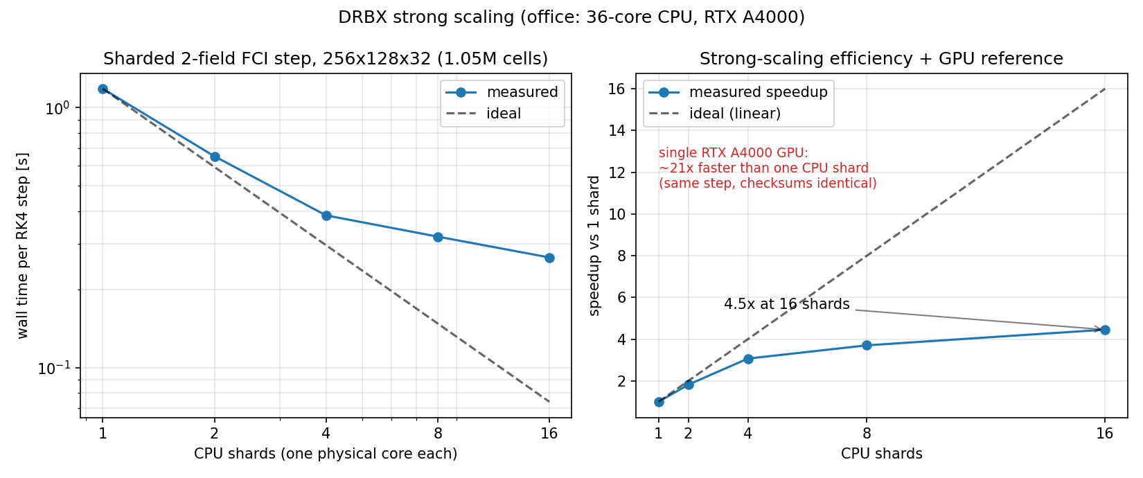
These ratios are lower than the earlier lineax-era curve (which reached 7.4x at 16) for a good reason: the single-device baseline is now much faster. The solvax GMRES potential solve and the sync-free RHS cut the per-step cost sharply, so the fixed halo-exchange cost is a larger fraction of a smaller total — there is less work left to parallelize. The absolute step time still improves monotonically with shard count.

On one NVIDIA RTX A4000 GPU the same step runs about 21x faster than a single core-bound CPU shard at grids that fit the GPU's constant-allocation limit (128 x 64 x 16: 6.6 ms vs 156 ms; 128 x 64 x 32: 13 ms vs 276 ms; checksums identical). The full 1.05M-cell grid overflows the single-GPU constant allocation, and running across the two A4000s trips a cross-device gather bug in the sharded halo path; both are documented limits, not supported claims (status as of 2026-07-18). The earlier "~96x" figure predates the CPU-baseline speedup and no longer holds against the faster baseline.

PYTHONPATH=src python examples/benchmarks/fci_sharded_strong_scaling.py

The demo writes its artifacts as scaling_<platform>.json and scaling_<platform>.png (one pair per host/platform), so CPU and GPU sweeps from different machines can coexist in the same output directory.

Current Fast Native Lanes¶

The strongest current native paths are the compact JAX-native field updates that stay inside jax.numpy kernels with lightweight analysis/output:

• anomalous diffusion (matrix-exponential propagator);
• electrostatic vorticity;
• Hasegawa-Wakatani drift-wave turbulence (pseudo-spectral);
• the reduced FCI operator and selected-field 3-D geometry kernels.

These are the best lanes for:

• performance measurements;
• precision studies;
• restart demonstrations;
• differentiable optimization loops.

Current End-To-End Differentiable Lanes¶

The intended end-to-end differentiable lane is:

• TOML deck or Python driver;
• native JAX field evolution;
• portable array payload;
• JAX-side objective or analysis functional.

The compact diffusion and vorticity kernels, the Hasegawa-Wakatani flagship, and the differentiable FCI drift-reduced RHS (native/fci_drb_rhs.py) are the best starting points today because they stay fully inside JAX.

The diffusion lane has committed focused differentiable examples:

• sensitivity analysis: examples/autodiff_diffusion_sensitivity.py
• inverse design: examples/autodiff_diffusion_inverse_design.py
• fixed-workload CPU/GPU scaling: examples/strong_scaling_diffusion.py

The current artifact bundle is documented in autodiff_and_scaling_examples.md.

The Hasegawa-Wakatani flagship is differentiable end-to-end, enabling gradient-based inverse design through turbulence; see Drift-Wave Turbulence. The FCI drift-reduced RHS is a PyTree that can be passed through jax.jvp, checked against finite differences, and matched under vmap, as documented in Stellarator FCI Validation.

Current Differentiable Example Results¶

On the committed diffusion examples:

• autodiff and finite-difference gradients match closely on the compact four-parameter sensitivity study;
• first-order autodiff uncertainty propagation agrees with the vectorized Monte Carlo comparison on the compact field and scalar quantities of interest;
• the inverse-design example reduces the objective from about 2.95e-3 to about 5.52e-5;
• the compact differentiable fixed-workload scaling artifact shows modest local CPU scaling on a MacBook: about 1.08x from 1 -> 2 and 1.10x from 1 -> 4 in process-group mode, and about 1.07x and 1.08x in host-device CPU pmap mode.

Those scaling numbers are intentionally framed narrowly: the compact diffusion curve is a differentiability and execution-mode check, not a headline performance claim, and it is measured on a differentiable objective rather than only on a forward solve.

What The Current Profiling Already Says¶

The committed profiling and runtime bundles already answer the first practical performance questions:

• avoid tiny per-field JIT dispatches on the reduced 3-D kernels;
• batch same-shape selected fields before entering the jitted kernel;
• warm once before timing;
• keep solver/case metadata out of static JIT arguments;
• keep file I/O, plotting, and JSON serialization outside hot kernels.

They also answer the first CPU-parallelism question:

• the default JAX CPU runtime appears as one CPU device and relies on XLA's internal CPU threading;
• explicit host-device CPU parallelism is possible by setting DRBX_HOST_DEVICE_COUNT=N before importing drbx or jax;
• on the committed differentiable diffusion scaling surface the local process-group mode is slightly stronger than the host-device pmap mode on this MacBook, but both are modest;
• CPU parallelization is real and usable here, but it should be treated as a bounded strong-scaling tool, not as an automatic replacement for accelerator execution.

Parallelization Model¶

There are three distinct execution modes worth separating:

• default CPU execution: one JAX CPU device with XLA-managed internal threading;
• explicit host-device CPU execution: multiple CPU devices exposed with DRBX_HOST_DEVICE_COUNT=N, then mapped with pmap or equivalent device-parallel transforms;
• process-group CPU execution: multiple Python workers with one JAX CPU device each.

The committed diffusion scaling artifact measures the last two explicitly, with the modest results quoted above.

Current GPU Status¶

The reachable office machine exposes two CUDA-visible JAX devices (RTX A4000, cuda:0 and cuda:1) with jax[cuda12]. Status as of 2026-07-18:

• single GPU: the sharded two-field step runs about 21x faster on one A4000 than on a single core-bound CPU shard at grids that fit the GPU's constant allocation (128 x 64 x 16: 6.6 ms vs 156 ms; 128 x 64 x 32: 13 ms vs 276 ms; checksums identical). The full 1.05M-cell grid overflows the single-GPU constant allocation (Failed to allocate ... for new constant);
• two GPUs: the 2-device sharded run currently fails in a cross-device gather inside the halo-exchange path; this bug is under investigation, so no 2-GPU scaling number is claimed;
• earlier small-kernel measurements (compact reduced lanes, ~1e-4 s warm executes) remain valid but are microbenchmarks, not whole-code claims.

Reproducible Profiling Workflow¶

The supported profiling entry point for the reduced FCI/geometry lanes is scripts/profile_stellarator_drb_pytree.py, which can collect cProfile output, JAX TensorBoard / Perfetto traces, device-memory profiles, persistent compilation-cache runs, and XLA dump trees. The workflow and recommended cases are documented in profiling_runtime.md.

4-Field Step: Fast Path, Whole-Step JIT, Coarse LU (2026-07-17)¶

Profiling the 4-field interchange RK4 step on the rotating ellipse at (24, 32, 8), single CPU, found the old eager default costing 1.200 s per step, of which roughly half was host-synced convergence checking in the perpendicular-Laplacian phi solver: the diagnostic path recomputes the true residual after each GMRES solve and converts residual norms and iteration counts to Python floats — about 490 device transfers per 4 steps (one batch per RK4 stage). Three changes landed in response, bringing the same step to 0.623 s per step (1.9x), with all 26 operator/turbulence/MMS/blob/sharded gates passing:

• phi-solver fast path: constructing PerpLaplacianInverseSolver with check_residual=False and calling it without return_diagnostics dispatches a jitted phi-only solve — no diagnostic matvecs, no residual floats, no host syncs — making the solver safe to call from inside jit-compiled stepping code. The diagnostic path is unchanged and remains the default for validation harnesses.
• whole-step JIT: the entire RK4 step — all four RHS evaluations, including their GMRES phi inversions — now compiles as one jit program in drbx.native.stellarator_turbulence.run_stellarator_turbulence (a one-time compile of about 9 s, then no per-stage Python dispatch). Supporting this, compute_2field_rhs / compute_4field_* now return timings=None by default (sync-free, jittable); passing with_diagnostics=True restores the host-synced stage-timings and phi-diagnostics payload the validation harnesses use.
• honored GMRES tolerance: the phi solve now honors the requested phi_inversion_tol — it was previously hardcoded to rtol=atol=1e-6, silently over-solving every stage for models that asked for a looser tolerance. Solvers constructed with the default tol=1e-6 are unchanged.

Additionally, build_perp_laplacian_mg_hierarchy now LU-factorizes the coarsest-level dense operator once at build time (jax.scipy.linalg.lu_factor, coarse systems up to 512 cells), so each V-cycle does a triangular solve instead of relying on coarse smoothing sweeps (see Solvers and Design Decisions).

JAX Ecosystem Usage¶

• solvax carries every structured solve: the FCI perpendicular-Laplacian inversion (solvax.gmres, restarted flexible GMRES over the matrix-free conservative operator — it replaced the earlier lineax backend on 2026-07-17 and measured ~1.8x faster per turbulence step), plus the Fourier–Helmholtz and tridiagonal solves.
• equinox and diffrax are still not used by any promoted kernel; they remain future options, not active dependencies.

Guidance For Users¶

If you need:

• the cleanest standalone runtime workflow: start from restartable_diffusion_tutorial.md;
• compact high-quality figures and movies: use validation_gallery.md;
• the best current base for differentiable research code: start from the compact native-exact diffusion and vorticity lanes, the Hasegawa-Wakatani flagship, or the differentiable FCI drift-reduced RHS.

Recommended Next Refactors¶

• keep expressing new physics directly on fixed-layout JAX-native arrays so the linearized residual does not need to reconstruct full guard-cell fields for each transform;
• fuse small same-shape analysis reductions where they currently enter JAX one field at a time;
• use more vmap-style batching where case structure is already homogeneous;
• keep plotting, output writing, and CLI serialization as boundary code rather than inside hot kernels;
• only widen equinox/diffrax usage where it removes a measured bottleneck.