Open-Field-Line SOL Flux Tube¶

The scrape-off layer (SOL) is the open-field-line region where field lines strike material target plates. drbx models it with an open slab flux tube: a straight field along the parallel coordinate z, bounded by targets at z = 0 and z = L_parallel, where a Bohm sheath drains the plasma at the sound speed. This is the open-field-line counterpart to the closed flux tubes (rotating ellipse, shifted torus, Hasegawa-Wakatani flux tube).

Geometry — open field lines¶

drbx.geometry.build_open_slab_geometry builds a Cartesian flux tube whose field lines are open: the forward field-line map exits the domain on the z = L target plane and the backward map on the z = 0 target plane, so the FCI endpoint masks (build_fci_target_masks) mark exactly the two target plates. These are the same masks the kept sheath / recycling closure compute_fci_sheath_recycling consumes: it applies a normalized Bohm flux n c_s on every target cell, the sheath heat transmission, and a recycled-neutral source, and it closes exact particle-recycling, zero-current, and neutral-energy accounting identities to machine precision.

Model — reduced isothermal SOL transport¶

drbx.native.sol_flux_tube evolves the parallel density n and momentum m = n v as an isothermal Euler system along the field,

d n / dt + d (n v) / dz = S_n
d m / dt + d (n v^2 + n c_s^2) / dz = 0

with an upstream particle source S_n and Bohm sheath outflow (|v| >= c_s) at the targets. Faces use a Rusanov flux; the update is pure JAX (jit/grad/vmap transparent).

What is checked¶

The gate tests/test_open_field_line_sol.py pins:

• the open geometry carries target endpoint masks on exactly the two target planes and nowhere else;
• the sheath / recycling closure closes its accounting identities to machine precision on this genuinely open geometry; and
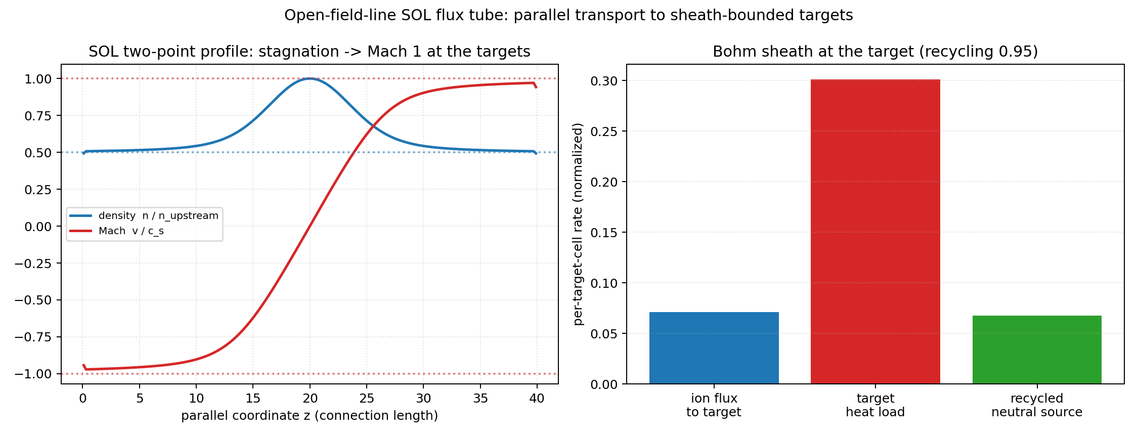
• the reduced SOL flux tube relaxes to the classic two-point steady state: the flow accelerates from a stagnation point to the sound speed (Mach 1) at each target, the target density is half the upstream density, and the upstream source exactly balances the total Bohm target loss.

The left panel of the figure shows that two-point profile (density falling to n_upstream / 2, Mach number rising from 0 to ±1 at the targets); the right panel shows the Bohm-sheath target diagnostics.

Reproduce¶

PYTHONPATH=src python examples/sol/open_sol_flux_tube.py
pytest -q tests/test_open_field_line_sol.py

The example is a flat script with every physics/numerics choice in the PARAMETERS block at the top (connection length, grid, source strength and width, CFL, recycling fraction). It prints stage-by-stage progress: a setup block (grid, timestep, integrated source), per-chunk relaxation lines with the target Mach numbers, the target/upstream density ratio, and the steady-state residual max|dn/dt|, and finally the sheath/recycling target accounting. A line-by-line walkthrough is in Tutorial: Building an Open SOL.