Autodiff And Scaling Examples
This page records the current focused differentiable examples and the current fixed-workload scaling artifact on the strongest compact native diffusion lane.
Why These Examples
Differentiable PDE and differentiable simulation workflows usually show three things first:
- direct sensitivity of a scalar objective to physical parameters
- uncertainty propagation from uncertain inputs to scalar and field quantities of interest
- inverse recovery of hidden parameters from a target state
- fixed-workload scaling of the gradient-enabled kernel
That is the surface used here too. It is the same general pattern used by projects such as JAX-FEM, JAX-MD, and the device-parallel mapping model documented in JAX pmap.
Scripts
- examples/autodiff_diffusion_sensitivity.py
- examples/autodiff_diffusion_uncertainty.py
- examples/autodiff_diffusion_inverse_design.py
- examples/strong_scaling_diffusion.py
- shared helper module: src/drbx/validation/autodiff_diffusion.py
- uncertainty helper module: src/drbx/validation/autodiff_diffusion_uncertainty.py
Sensitivity Analysis
Run:
PYTHONPATH=src .venv/bin/python examples/autodiff_diffusion_sensitivity.py
Outputs:
- analysis JSON:
docs/data/autodiff_diffusion_sensitivity_artifacts/data/autodiff_diffusion_sensitivity_analysis.json(written when you run the script) - figure: media/autodiff_sensitivity.png
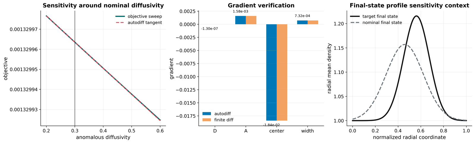
Current committed result:
- autodiff and finite-difference gradients agree closely on all four design parameters
- the center parameter is the dominant sensitivity on this setup
- the diffusivity tangent matches the explicit sweep in the local neighborhood
Uncertainty Quantification
Run:
PYTHONPATH=src .venv/bin/python examples/autodiff_diffusion_uncertainty.py
Outputs:
- analysis JSON:
docs/data/autodiff_diffusion_uncertainty_artifacts/data/autodiff_diffusion_uncertainty_analysis.json(written when you run the script) - arrays NPZ: release-hosted (
docs__data__autodiff_diffusion_uncertainty_artifacts__data__autodiff_diffusion_uncertainty_arrays.npzon thevalidation-artifacts-2026-04-28release; requires repository access) - figure: media/autodiff_uncertainty.png
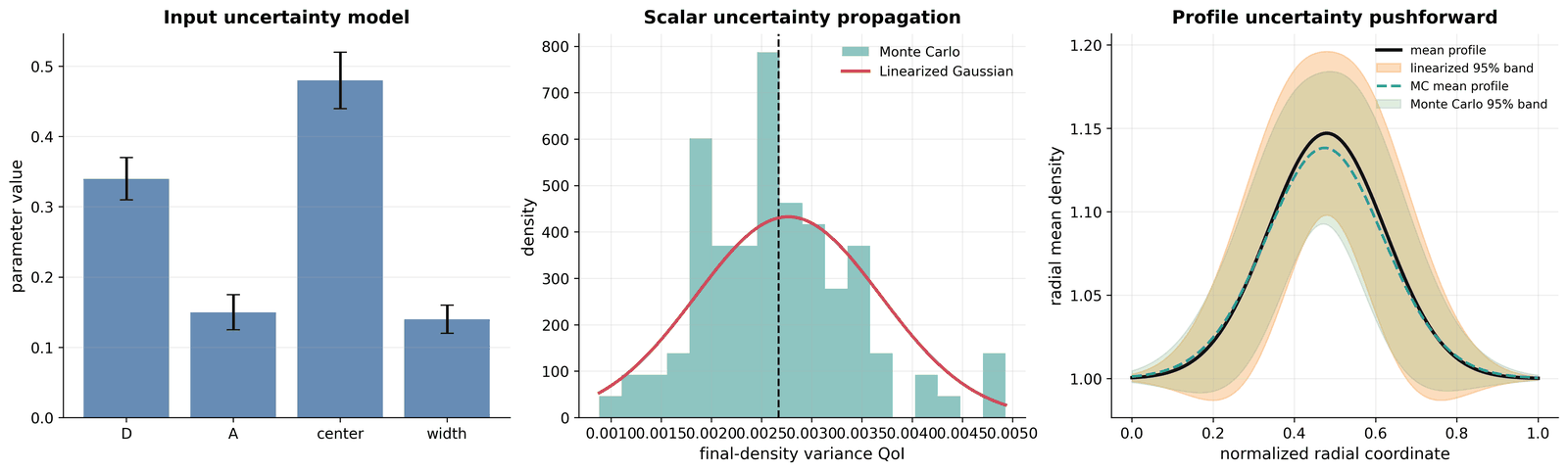
Current committed result:
- the scalar quantity of interest uses the final active-domain density variance on the same compact native diffusion lane;
- the field quantity of interest uses the radial mean of the final active-domain density;
- first-order autodiff covariance pushforward and vectorized Monte Carlo stay close on both the scalar QoI and the profile uncertainty band;
- this gives the differentiable lane a standard UQ example rather than stopping at gradients and inverse design only.
Inverse Design
Run:
PYTHONPATH=src .venv/bin/python examples/autodiff_diffusion_inverse_design.py
Outputs:
- analysis JSON:
docs/data/autodiff_diffusion_inverse_design_artifacts/data/autodiff_diffusion_inverse_design_analysis.json(written when you run the script) - figure: media/autodiff_inverse_design.png
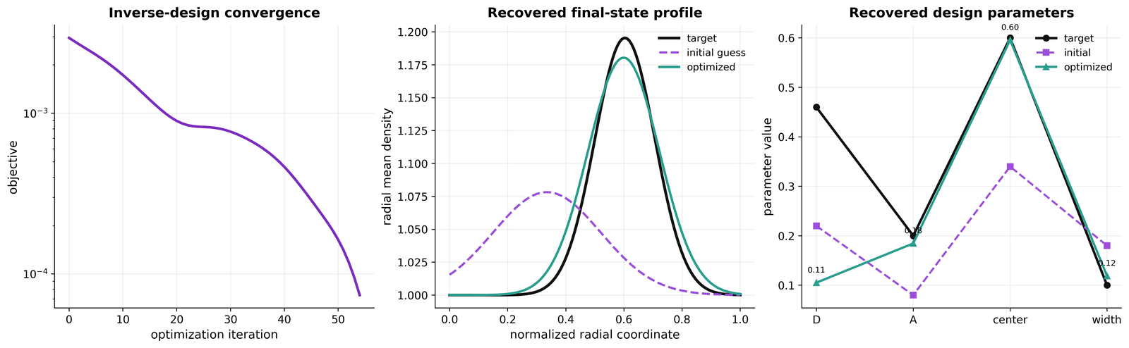
Current committed result:
- the objective drops from about
2.95e-3to about5.52e-5 - the optimized final-state profile nearly overlays the target profile
- the optimized design parameters recover the dominant target structure cleanly
Strong Scaling
Run locally on CPU only:
PYTHONPATH=src python examples/strong_scaling_diffusion.py
Like every example, the script has no command-line flags — the sweep is configured by the PARAMETERS constants near the top:
CPU_DEVICE_COUNTS = (1, 2, 4)— laptop-sized sweep; office-scale runs use(1, 2, 4, 8);TOTAL_BATCH = 16— fixed global workload (must divide by every device count), which is what makes this a strong-scaling plot;NX,NY,STEPS,REPEATS— per-sample workload and timing repeats;RUN_REMOTE_GPU = False— setTrueto add remote-GPU points over SSH, withGPU_DEVICE_COUNTS = (1, 2)andREMOTE_HOSTnaming the machine.
The CPU artifact measures two distinct local modes:
process_group: one Python worker per CPU partitionhost_pmap: one process withDRBX_HOST_DEVICE_COUNT=Nand device-parallelpmap
To inspect the runtime mode directly in a fresh process:
DRBX_HOST_DEVICE_COUNT=4 PYTHONPATH=src python - <<'PY'
from drbx.runtime import runtime_parallel_summary
import json
print(json.dumps(runtime_parallel_summary(), indent=2, sort_keys=True))
PY
Outputs:
- analysis JSON:
docs/data/strong_scaling_diffusion_artifacts/data/strong_scaling_diffusion_analysis.json(written when you run the script) - figure: media/strong_scaling_diffusion.png
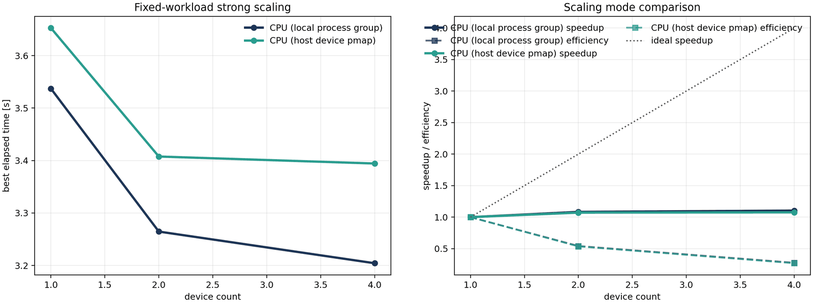
Current committed result:
- local CPU process-group reference on the heavier medium workload:
- about
3.54 s -> 3.26 s -> 3.20 s - about
1.08xfrom1 -> 2 - about
1.10xfrom1 -> 4 - local CPU host-device
pmapon the same workload: - about
3.65 s -> 3.41 s -> 3.39 s - about
1.07xfrom1 -> 2 - about
1.08xfrom1 -> 4 - the current committed artifact was regenerated locally with
RUN_REMOTE_GPU = False, so the figure emphasizes the two CPU modes on this MacBook rather than repeating the earlier remote GPU line
Interpretation:
- several CPU cores can be used on this machine in both execution modes
- on the currently committed heavier workload, the local process-group mode is slightly better than host-device
pmap, but both CPU curves are modest - explicit host-device
pmapis still a real supported mode, but it is not a strong-scaling headline result on this benchmark - the honest conclusion on this MacBook is that CPU parallelism is available and measurable, but the reviewer-facing strong-scaling claim should still stay bounded
- all curves are measured on a differentiable objective, not just a forward solve
Notes On Method
- the objective is evaluated on the compact native diffusion lane because it is already JAX-native and differentiable end to end
- the CPU benchmark uses one JAX worker process per local worker to avoid oversubscribing host threads
- the explicit host-device CPU benchmark uses
DRBX_HOST_DEVICE_COUNT=Nto expose multiple CPU devices before import, then maps the objective withpmap - the optional GPU benchmark uses
pmapon the remote two-GPU machine - the total workload is held fixed, so the figure is a strong-scaling plot rather than a throughput plot
Follow-On Work
The next higher-value differentiable examples should be:
- vorticity or drift-wave sensitivity/UQ of a scalar QoI
- an inverse-design example with boundary/source controls rather than only initial-condition controls
- memory and compilation-cache measurements alongside the current timing plot