Tutorial: Building an Open SOL — Sheath, Neutrals, Detachment¶

This tutorial builds up the scrape-off-layer (SOL) physics ladder in three steps, each one a runnable example:

1. an open flux tube with Bohm sheath targets (examples/sol/open_sol_flux_tube.py);
2. add neutrals and recycling with the hermes-3 atomic reactions (examples/sol/recycling_sol.py);
3. evolve the temperature and reach detachment — the SD1D target-flux rollover (examples/benchmarks/b6_detachment_rollover.py).

The equations for each stage are on Models and Governing Equations; physics pages: Open-Field-Line SOL and Neutrals and Recycling.

Step 1 — the open flux tube and the two-point steady state¶

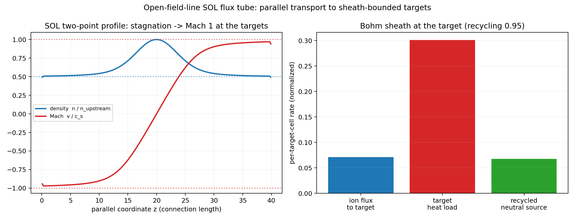
An "open" geometry is one whose field lines terminate on material targets. In drbx that is a property of the FCI maps, not a special coordinate system:

from drbx.geometry import build_open_slab_geometry

geometry = build_open_slab_geometry(SHAPE, parallel_length=PARALLEL_LENGTH)

with SHAPE = (1, 1, 200) — one flux tube, 200 parallel cells — and PARALLEL_LENGTH = 40.0 (the target-to-target connection length, normalized). The forward field-line map exits the domain at z = L and the backward map at z = 0, so the FCI endpoint masks mark exactly the two target planes. Every open-field-line closure in the package keys off these masks.

The model parameters are one dataclass:

params = SolFluxTubeParameters(
    sound_speed=1.0,        # isothermal c_s; sets the Bohm outflow speed
    source_amplitude=0.02,  # peak of the Gaussian upstream particle source
    source_width=4.0,       # parallel 1/e width of the source
    density_floor=1e-6,     # positivity floor applied after each RK4 step
)
source = sol_flux_tube_source(geometry, params)   # Gaussian at the midplane
density = jnp.ones(geometry.shape)                # uniform start, at rest
momentum = jnp.zeros(geometry.shape)

Why these values: the source is weak (0.02) so the steady state stays in the quasi-linear two-point regime where the analytic prediction (\(n_{\mathrm{target}} = n_{\mathrm{upstream}}/2\), Mach 1 at the plates) holds; the width 4.0 localizes it upstream without making the profile a delta function. The timestep is a CFL choice against the fastest wave (\(|v| + c_s \le 2 c_s\) near the targets):

dt = CFL * dz / (SOUND_SPEED + 1.0)   # CFL = 0.4

and STEPS = 60000 RK4 steps is simply long enough (hundreds of sound times) for the residual max|dn/dt| to fall many decades. The run loop prints, per chunk, the target Mach numbers (→ ±1), the density ratio (→ 0.5), and the residual. Finally the sheath/recycling closure audits the relaxed state:

sheath = compute_fci_sheath_recycling(
    density, te, ti, geometry.maps, recycling_fraction=0.95
)

With TE = TI = 0.5 the sheath sound speed \(\sqrt{T_e + T_i} = 1\) matches the transport model's c_s, so the Bohm flux the closure reports equals the flux the flux tube actually drained — and the particle-recycling and zero-current identities close to ~1e-16. Run it:

PYTHONPATH=src python examples/sol/open_sol_flux_tube.py

Step 2 — neutrals, recycling, and the onset of detachment¶

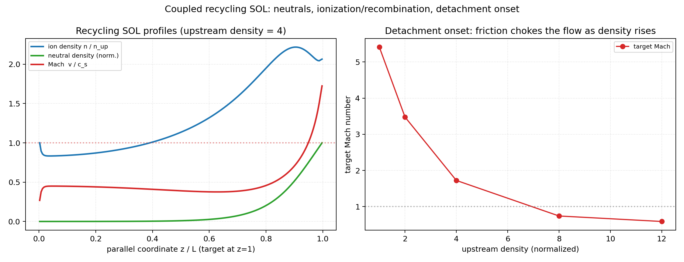
Real targets are not perfect absorbers: most of the ion flux returns as neutral gas, which diffuses upstream, ionizes where the plasma is hot, and drags the flow by charge exchange. The coupled model is drbx.native.neutrals.recycling_sol_model, and the example drives it half-domain (stagnation midplane at z = 0, one target at z = L):

params = SolRecyclingParameters(
    parallel_length=30.0,      # metres — sets the *physical* atomic-rate scale
    upstream_density=4.0,      # normalized; Dirichlet-pinned at z = 0
    recycling_fraction=0.95,   # R: fraction of target ion flux returned as neutrals
    neutral_diffusion=8.0,     # parallel diffusion enhancement (kinetic proxy)
    neutral_temperature=0.04,  # ~2 eV Franck-Condon neutrals (normalized to 100 eV)
    ion_mass=2.0,              # deuterium
    normalization=PlasmaNormalization(),   # Nnorm = 1e19 m^-3, Tnorm = 100 eV
)

Parameter reasoning:

• parallel_length is in metres because the AMJUEL rate fits take physical \(T_e\) [eV] and \(n_e\) [m⁻³]: the connection length fixes how many ionization mean-free-paths fit in the tube.
• The temperature profile is prescribed (UPSTREAM_EV = 30, TARGET_EV = 1.5, quadratic in between via linear_target_temperature_profile): hot attached upstream, cold recycling region at the plate. Imposing \(T(z)\) sidesteps the stiff conduction/radiation energy balance — that is exactly what Step 3 adds.
• recycling_fraction = 0.95 is a typical divertor value (5% pumped); 1.0 gives a fully recycling target, 0.0 recovers Step 1.
• neutral_diffusion = 8.0 enhances the fluid neutral diffusivity as a proxy for kinetic neutral transport (hermes-3 practice).
• DT = 0.3 * (1/NZ) / 3: CFL 0.3 against the fastest normalized wave (~3 c_s); the stiff pieces (neutral diffusion, ionization) are implicit (solvax tridiagonal + per-cell implicit update), so the CFL only has to cover the hyperbolic transport.

The script relaxes a reference case, printing the target Mach number, target flux, and neutral cushion per chunk, then scans UPSTREAM_SCAN = [1, 2, 4, 8, 12]. The physics to watch: as upstream density rises, charge-exchange + recombination friction chokes the flow — the target Mach number falls toward and below 1. That is the onset of detachment, with the temperature still held fixed.

PYTHONPATH=src python examples/sol/recycling_sol.py

Step 3 — evolved temperature and the detachment rollover¶

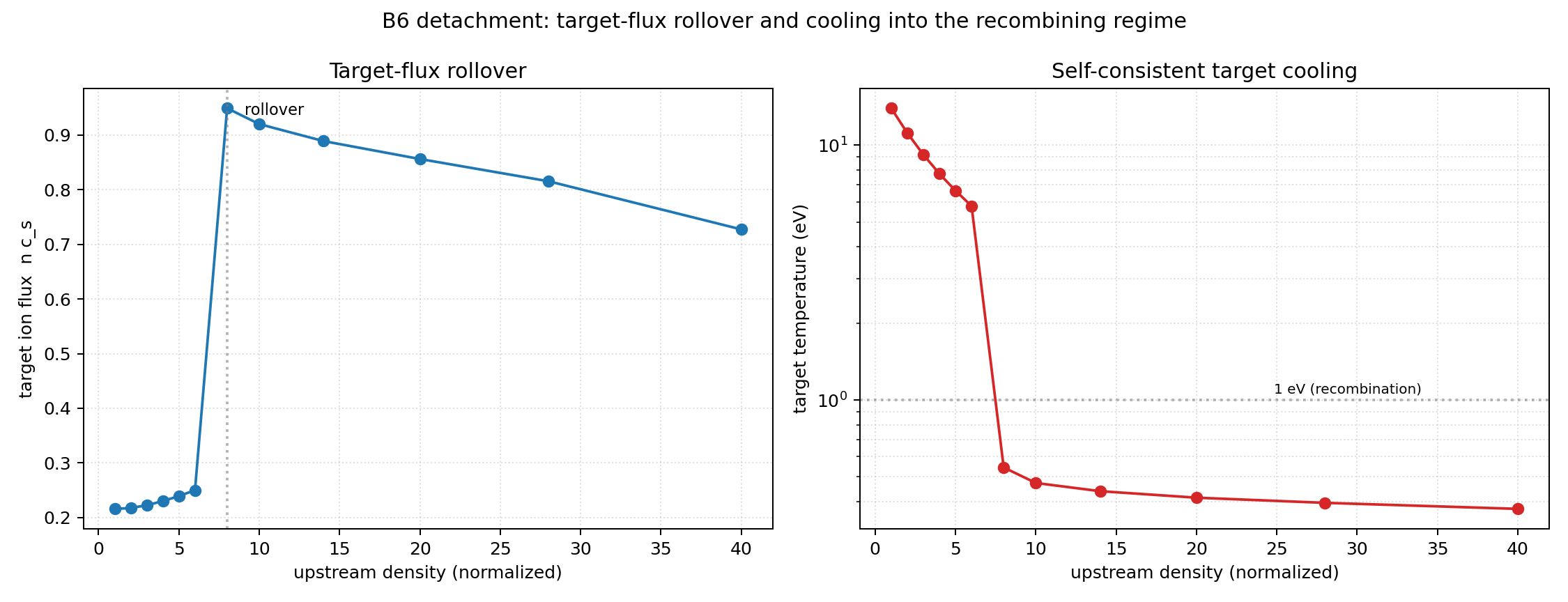
Detachment proper needs the target temperature to respond: cooling raises recombination, which removes plasma before it reaches the plate, which cools the target further. detachment_sol_model adds the plasma pressure equation with three stiff ingredients, each handled implicitly:

params = DetachmentSolParameters(
    parallel_length=30.0,
    upstream_density=upstream,      # the scan variable
    upstream_power=6.0,             # fixed: this is a density scan at constant power
    power_width=0.2,                # power deposited in the upstream 20% of the tube
    conduction_coefficient=2.0,     # Spitzer kappa0: q = -kappa0 T^{5/2} dT/dz
    sheath_transmission=7.0,        # gamma: Bohm heat sink gamma n c_s T at the target
    recycling_fraction=0.95,
    neutral_diffusion=8.0,
    ion_mass=2.0,
    normalization=PlasmaNormalization(Tnorm=50.0),   # SOL reference: 50 eV
)

• Implicit Spitzer conduction \(\kappa \sim T^{5/2}\): a solvax tridiagonal solve per step, because explicit parabolic conduction at \(T^{5/2}\) stiffness would force a hopeless timestep.
• Self-limiting radiation: the AMJUEL radiative/ionization energy loss is applied as \(P \leftarrow P/(1 + \Delta t\, \mathrm{rate})\) — it can never drive \(P < 0\) and switches itself off as the plasma cools past the radiation peak.
• sheath_transmission = 7.0 is the standard total sheath heat transmission \(\gamma \approx 7\) for \(T_e = T_i\) hydrogen.
• Tnorm = 50 eV centers the normalization on SOL temperatures so the detachment transition (~1 eV) is well-resolved numerically.

The scan DENSITY_SCAN = [1 ... 40] relaxes each upstream density from a cold start (INITIAL_TEMPERATURE = 0.6, i.e. 30 eV) for 45,000 operator-split steps and records the target flux and temperature. The two signatures of the SD1D benchmark (Dudson et al., PPCF 61, 065008 (2019)) appear: the target ion flux rises then rolls over, and the target temperature crosses 1 eV into the recombining regime.

PYTHONPATH=src python examples/benchmarks/b6_detachment_rollover.py

Coda — controlling detachment with a gradient¶

The entire detaching solve is differentiable, so "find the upstream density that puts the target exactly at 1 eV" is a Newton iteration on \(T_{e,\mathrm{target}}(n_{\mathrm{up}})\) with the sensitivity from forward-mode autodiff through the full stiff solve:

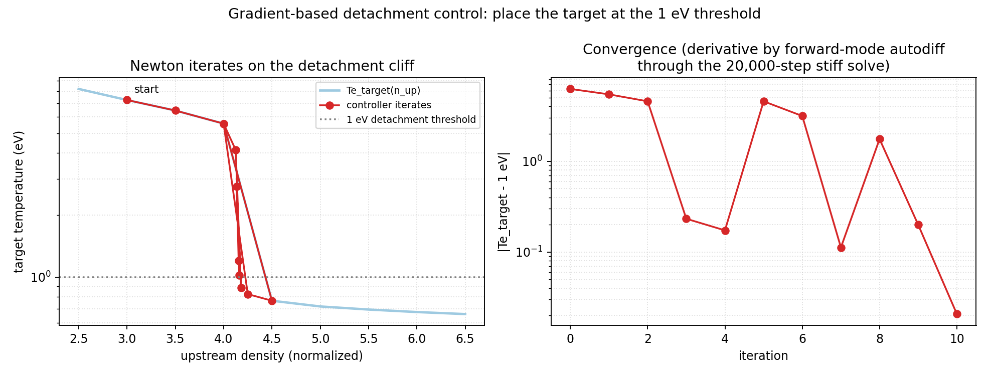
See examples/autodiff/detachment_control.py and the write-up on Neutrals and Recycling. Gates for everything in this tutorial: tests/test_open_field_line_sol.py, tests/test_native_recycling_sol.py, tests/test_native_detachment_sol.py, tests/test_detachment_control.py.