The Linearized Drift-Reduced Braginskii Solver¶

drbx.linear answers the first question asked of any plasma model: given an equilibrium, which perturbations grow, and how fast?

What is solved¶

Linearizing a model about an equilibrium u0 gives

d(delta u)/dt = A delta u,        A = d rhs / d u |_(u0)

Writing a perturbation as delta ~ exp(lambda t), the eigenvalues lambda = gamma + i Omega of A give the growth rate gamma = Re(lambda) and the oscillation frequency |Omega| of every eigenmode.

How it is solved¶

Two entry points, one engine:

Analytic dispersion operators — for a single Fourier mode of a reduced model, A is a small complex matrix written down from the linearized equations (resistive_drift_wave_operator, shear_alfven_operator, interchange_operator in linear/dispersion.py). Because the operators are assembled from the model equations, diagonalizing them reproduces the analytic dispersion relations rather than having those relations wired in.
The general engine — jacobian_operator(rhs, equilibrium) builds A from any right-hand side with jax.jacfwd (no hand derivation), and eigenmodes(A) returns growth rates, frequencies, and eigenvectors sorted by growth (linear/eigen.py). States must be real; complex spectral states are realified first (the pattern used in the Hasegawa-Wakatani gate below).

Regimes and literature anchors¶

Linear DRB survey

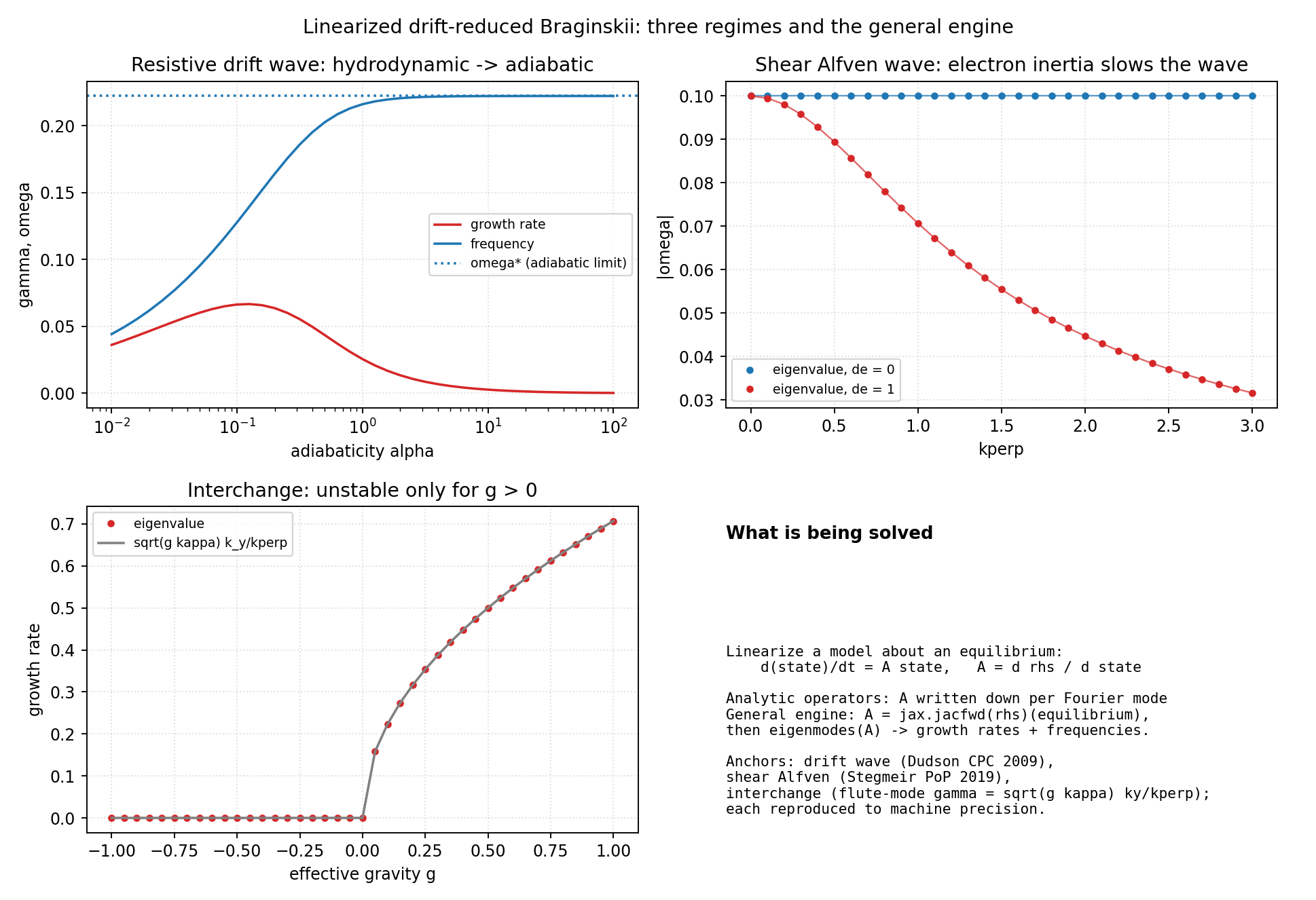
Regime	Physics	Analytic limit reproduced	Reference
Resistive drift wave, hydrodynamic (`alpha << 1`)	weak parallel coupling; resistive branch grows	growth rises toward the hydrodynamic regime	Dudson et al., CPC 180, 1467 (2009); Hasegawa & Wakatani, PRL 50, 682 (1983)
Resistive drift wave, adiabatic (`alpha >> 1`)	electrons force `n ~ phi`; a propagating drift wave	`omega -> omega* = kappa k_y / (1 + kperp^2)`	Dudson et al., CPC 180, 1467 (2009)
Shear Alfven wave (`d_e = 0`)	ideal field-line bending	`omega = k_par v_A`	Stegmeir et al., PoP 26, 052517 (2019)
Shear Alfven with electron inertia	finite electron mass slows the wave	`omega = k_par v_A / sqrt(1 + kperp^2 d_e^2)`	Stegmeir et al., PoP 26, 052517 (2019)
Interchange, stable (`g kappa < 0`)	curvature and gradient oppose (good curvature)	`gamma = 0` (stable oscillation)	flute-mode theory
Interchange, unstable (`g kappa > 0`)	curvature drives the gradient (bad curvature)	`gamma = sqrt(g kappa) k_y / kperp`, flute (`k_x -> 0` largest)	flute-mode theory; the linear physics behind SOL blobs

Every row is reproduced to machine precision (1e-12 to 1e-16) in tests/test_linear_dispersion.py (24 tests), and surveyed with printed explanations in examples/benchmarks/linear_drb_survey.py; the compact two-panel version is examples/benchmarks/linear_dispersion.py.

Geometries¶

The dispersion operators above live on a periodic slab flux tube (the Hasegawa-Wakatani setting). The same linearization machinery is exercised on curved and non-axisymmetric geometry elsewhere in the suite:

The real nonlinear model. The general engine linearizes the full pseudo-spectral Hasegawa-Wakatani model (realified spectral state) and recovers the analytic single-mode operator to ~1e-15 (test_general_engine_linearizes_the_hasegawa_wakatani_model) — the check that jacobian_operator is trustworthy on production right-hand sides.
Helical flux tube. A single Fourier mode of the nonlinear Hasegawa-Wakatani model grows at the resistive drift-wave operator's eigenvalue to ~1e-14 (tests/test_hasegawa_wakatani.py), tying the nonlinear code to the linear solver; the drift-reduced FCI operator stack carries the same curvature terms on the shifted-torus helical geometry.
Rotating-ellipse stellarator. The small-amplitude response on the genuinely non-axisymmetric metric is pinned by the differentiable rollout gates: the gradient of an evolved diagnostic matches finite differences (tests/test_rotating_ellipse_fci.py), which is the linearized response computed two independent ways.

Using it¶

from drbx.linear import jacobian_operator, eigenmodes

operator = jacobian_operator(my_rhs, my_equilibrium)   # A = d rhs / d u
modes = eigenmodes(operator)                           # sorted by growth rate
print(modes.growth_rates[0], modes.frequencies[0])     # the fastest mode

Reproduce¶

PYTHONPATH=src python examples/benchmarks/linear_drb_survey.py       # full survey
PYTHONPATH=src python examples/benchmarks/linear_dispersion.py  # compact B2/B3
pytest -q tests/test_linear_dispersion.py